Introductory MAZE Tutorial
These tutorials showcase the capabilities of the MAZE code, along with comments describing how to use the functions shown in the demos.
Verify Installation
Verify the installation by importing maze and making a simple empty Zeolite
import maze
maze.Zeolite()
Zeolite(symbols='', pbc=False)
Cif Fetching from the Database of Zeolite Structures
The database of zeolite structures is a useful resource for zeolite simulation experiments. It contains cif files for all synthesized zeolites, organized by their three letter zeolite code. Downloading them from the website is easy when working on a local machine, but challenging when working on a remote machine. To facilitate smoother workflows, a simple python function which downloads cif files from the database was created. An example of using this to download a few different cif files is shown below.
Note: Some users have had trouble using the cif_download function and the make method. The cause of this issue is typically latency issues with the IZA database’s website. If you encounter these issues you can download all of the CIF files in the database by going to this google drive link, downloading the zip folder and extracting the data folder. Place this data folder in your working directory. You can see your working directory by running the python command import os followed by print(os.getcwd()). After placing the data folder, which contains all of the CIF files from the IZA database, in your working directory, you will be able to run the make command without accessing the IZA database.
Note: The CIF reading capabilities of MAZE rely on those of ASE. Version 3.21.0 of ASE introduced a refactored CIF reader, which is not able to read all of the CIF files on the IZA database, thus most, but not all of the CIF files in the IZA database are readable with MAZE and the most recent version of ASE. This issue can be mitigated by using MAZE with any ASE version < 3.21.0, which is able to read and label the T-sites of all of the CIF files in the IZA database. This issuse might be fixed in future versions of ASE.
First, we import the MAZE package, the glob package, and the download_cif function from the maze.cif_download module.
>>> import maze
>>> from maze.cif_download import download_cif
>>> import glob
Next, we declare a helper function which prints out all of the directories in the current working directory. This will help us visualize the download_cif function’s behavior.
>>> def print_dirs():
...     print('dirs in cwd',  glob.glob('**/'))
...
We can view the directories names in our current directory using our helper function.
>>> print_dirs()
dirs in cwd []
Now, let’s download the GOO cif file, using the download_cif function. By default, the cif file is downloaded to the data directory; if this ‘data’ directory doesn’t exist, it is created.
>>> download_cif("GOO") # downloads "GOO.cif" to data/GOO.cif
>>> print_dirs()
dirs in cwd ['data/']
>>> print('files in data dir', glob.glob("data/*"))
files in data dir ['data/goo.cif']
We can download the cif file to a custom location by specifying the directory we want to use:
>>> download_cif("off", data_dir="my_other_data")
>>> print_dirs()
dirs in cwd ['my_other_data/', 'data/']
>>> print('files in my_other_data dir', glob.glob("my_other_data/*"))
files in my_other_data dir ['my_other_data/off.cif']
Making a Zeolite Using the Make Function
A cif file contains the crystallographic information that defines a zeolite structure. A downloaded cif from the iza-sc database of zeolite strucutres looks like this:
#**************************************************************************
#
# cif taken from the iza-sc database of zeolite structures
# ch. baerlocher and l.b. mccusker
# database of zeolite structures: http://www.iza-structure.org/databases/
#
# the atom coordinates and the cell parameters were optimized with dls76
# assuming a pure sio2 composition.
#
#**************************************************************************

_cell_length_a                  13.6750(0)
_cell_length_b                  13.6750(0)
_cell_length_c                  14.7670(0)
_cell_angle_alpha               90.0000(0)
_cell_angle_beta                90.0000(0)
_cell_angle_gamma              120.0000(0)

_symmetry_space_group_name_h-m     'r -3 m'
_symmetry_int_tables_number         166
_symmetry_cell_setting             trigonal

loop_
_symmetry_equiv_pos_as_xyz
'+x,+y,+z'
'2/3+x,1/3+y,1/3+z'
'1/3+x,2/3+y,2/3+z'
'-y,+x-y,+z'
... skipping all of this info for space
...

loop_
_atom_site_label
_atom_site_type_symbol
_atom_site_fract_x
_atom_site_fract_y
_atom_site_fract_z
    o1    o     0.9020    0.0980    0.1227
    o2    o     0.9767    0.3101    0.1667
    o3    o     0.1203    0.2405    0.1315
    o4    o     0.0000    0.2577    0.0000
    t1    si    0.9997    0.2264    0.1051
An important piece of information in each cif file is the
_atom_site_label (01, 02, … t1, t2.. ect.) that is located in the first
column near the atom position information. This information about the
atoms identities is lost when the ase.io.read function is used to
build an atoms object from a cif file. Because the identity of the
T-sites is critical for zeolite simulation experiments, this issue
inspired the creation of a custom constructor of the Zeolite object:
make. This static method creates a Zeolite object, labels the
unique atoms by tagging them, and then stores the mapping between the
atom_site_label and the atom indices in the dictionaries
site_to_atom_indices and atom_indices_to_site.
To demonstrate this feature, let us try building a Zeolite object
from a cif file.
First, we import the MAZE package, the cif_download function and the Zeolite object
import maze
from maze.cif_download import download_cif
Next we import some ase packages to help us view the Zeolites we make.
import matplotlib.pyplot as plt
from ase.visualize.plot import plot_atoms
First we use the download_cif function to fetch the CHA.cif file from the IZA database.
download_cif('CHA', data_dir='data')
Now we can use the static make method to Zeolite with labeled
atoms.
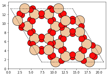
Our Zeolite object has been built. We can view it with the ase
plot_atoms method (or view method). This works flawlessly because the
Zeolite class is a subclass of the Atoms class.
plot_atoms(cha_zeolite)
The atom identity information is stored in two dictionaries. Let’s take a look at them:
print(cha_zeolite.site_to_atom_indices)
{'O1': [0, 1, 2, 3, 4, 5, 6, 7, 8, 9, 10, 11, 12, 13, 14, 15, 16, 17], 'O2': [18, 19, 20, 21, 22, 23, 24, 25, 26, 27, 28, 29, 30, 31, 32, 33, 34, 35], 'O3': [36, 37, 38, 39, 40, 41, 42, 43, 44, 45, 46, 47, 48, 49, 50, 51, 52, 53], 'O4': [54, 55, 56, 57, 58, 59, 60, 61, 62, 63, 64, 65, 66, 67, 68, 69, 70, 71], 'T1': [72, 73, 74, 75, 76, 77, 78, 79, 80, 81, 82, 83, 84, 85, 86, 87, 88, 89, 90, 91, 92, 93, 94, 95, 96, 97, 98, 99, 100, 101, 102, 103, 104, 105, 106, 107]}
print(cha_zeolite.atom_indices_to_sites)
{0: 'O1', 1: 'O1', 2: 'O1', 3: 'O1', 4: 'O1', 5: 'O1', 6: 'O1', 7: 'O1', 8: 'O1', 9: 'O1', 10: 'O1', 11: 'O1', 12: 'O1', 13: 'O1', 14: 'O1', 15: 'O1', 16: 'O1', 17: 'O1', 18: 'O2', 19: 'O2', 20: 'O2', 21: 'O2', 22: 'O2', 23: 'O2', 24: 'O2', 25: 'O2', 26: 'O2', 27: 'O2', 28: 'O2', 29: 'O2', 30: 'O2', 31: 'O2', 32: 'O2', 33: 'O2', 34: 'O2', 35: 'O2', 36: 'O3', 37: 'O3', 38: 'O3', 39: 'O3', 40: 'O3', 41: 'O3', 42: 'O3', 43: 'O3', 44: 'O3', 45: 'O3', 46: 'O3', 47: 'O3', 48: 'O3', 49: 'O3', 50: 'O3', 51: 'O3', 52: 'O3', 53: 'O3', 54: 'O4', 55: 'O4', 56: 'O4', 57: 'O4', 58: 'O4', 59: 'O4', 60: 'O4', 61: 'O4', 62: 'O4', 63: 'O4', 64: 'O4', 65: 'O4', 66: 'O4', 67: 'O4', 68: 'O4', 69: 'O4', 70: 'O4', 71: 'O4', 72: 'T1', 73: 'T1', 74: 'T1', 75: 'T1', 76: 'T1', 77: 'T1', 78: 'T1', 79: 'T1', 80: 'T1', 81: 'T1', 82: 'T1', 83: 'T1', 84: 'T1', 85: 'T1', 86: 'T1', 87: 'T1', 88: 'T1', 89: 'T1', 90: 'T1', 91: 'T1', 92: 'T1', 93: 'T1', 94: 'T1', 95: 'T1', 96: 'T1', 97: 'T1', 98: 'T1', 99: 'T1', 100: 'T1', 101: 'T1', 102: 'T1', 103: 'T1', 104: 'T1', 105: 'T1', 106: 'T1', 107: 'T1'}
Depending on the situation, one dictionary may be more useful than the other.
One Step Zeolite Construction
Downloading a cif file everytime you want to load a new Zeolite can be
annoying. Thus, the make function automatically downloads the cif
file from the IZA database if it cannot be located in the provided
directory. It places the downloaded cif file in folder called data
in the current working directory. Data paths can be specified with the
data_dir optional argument.
from maze import Zeolite
bea_zeolite = Zeolite.make('BEA')  # Download the BEA cif file and build zeolite
plot_atoms(bea_zeolite)
Identifying Atom Types in a Zeolite Structure
The Zeotype class includes methods for identifying the different
types of atoms in a zeolite structure. These methods will work on all
Zeotype objects, even those where the atom_indices_to_site and
site_to_atom_indices are not set.
Let’s import the Zeolite object and make a BEA structure and some tools to visualize the structures we create.
from maze import zeolite
import matplotlib.pyplot as plt
from ase.visualize.plot import plot_atoms
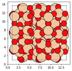
bea_zeolite = Zeolite.make('BEA')
plot_atoms(bea_zeolite)

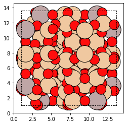
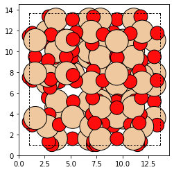
To make things more interesting, let us replace the Si-T1 sites in the bea Zeolite with Aluminum.
for t1_index in bea_zeolite.site_to_atom_indices['T1']:
    bea_zeolite[t1_index].symbol = 'Al'
plot_atoms(bea_zeolite)
Making a replacement is that simple! Now we will use the
count_elements method to get the count of each atom in the zeolite
and the idenity of each atom.
atoms_indices, count = bea_zeolite.count_elements()
print(atoms_indices)
{'O': [0, 1, 2, 3, 4, 5, 6, 7, 8, 9, 10, 11, 12, 13, 14, 15, 16, 17, 18, 19, 20, 21, 22, 23, 24, 25, 26, 27, 28, 29, 30, 31, 32, 33, 34, 35, 36, 37, 38, 39, 40, 41, 42, 43, 44, 45, 46, 47, 48, 49, 50, 51, 52, 53, 54, 55, 56, 57, 58, 59, 60, 61, 62, 63, 64, 65, 66, 67, 68, 69, 70, 71, 72, 73, 74, 75, 76, 77, 78, 79, 80, 81, 82, 83, 84, 85, 86, 87, 88, 89, 90, 91, 92, 93, 94, 95, 96, 97, 98, 99, 100, 101, 102, 103, 104, 105, 106, 107, 108, 109, 110, 111, 112, 113, 114, 115, 116, 117, 118, 119, 120, 121, 122, 123, 124, 125, 126, 127], 'Al': [128, 129, 130, 131, 132, 133, 134, 135], 'Si': [136, 137, 138, 139, 140, 141, 142, 143, 144, 145, 146, 147, 148, 149, 150, 151, 152, 153, 154, 155, 156, 157, 158, 159, 160, 161, 162, 163, 164, 165, 166, 167, 168, 169, 170, 171, 172, 173, 174, 175, 176, 177, 178, 179, 180, 181, 182, 183, 184, 185, 186, 187, 188, 189, 190, 191]}
print(count)
{'O': 128, 'Al': 8, 'Si': 56}
Extracting, Adding and Capping Clusters
One of the most useful features of the MAZE package is the ability to
add and remove atoms from a Zeolite object. To demonstrate this, we
will extract a cluster from an Zeolite object, change some of the
atoms, and then integrate it back into the main Zeolite.
First, we import the zeolite object and the plot_atoms function.
from maze import zeolite
import matplotlib.pyplot as plt
from ase.visualize.plot import plot_atoms
Then we make a bea_zeolite object
bea_zeolite = Zeolite.make('BEA')
plot_atoms(bea_zeolite)

The next step is to pick a T-site and then use one of the static methods
in the Cluster class to select indices to build the cluster.
The atom 154 is right in the middle of the zeolite, which will make
viewing the cluster creation easy. One could also use the
site_to_atom_indices dictionary to select a specific T site.
The Zeolite object uses a ClusterMaker object to select out certain
groups of atoms from the Zeolite.
By default a DefaultClusterMaker object is used. This
DefaultClusterMaker object has a get_cluster_indices method
which uses get_oh_cluster_indices function to selects the indices of
central t atom, and surrounding oxygens and hydrogens. There are other
cluster functions avalible in the source code of
DefaultClusterMaker. If you need some different functionality,
simply make your own ClusterMaker object and set the
Zeolite.cluster_maker attribute to your custom cluster maker.
Let us call our bea_zeolite’s ClusterMaker object’s
get_cluster_indices fun, to see what indices it will select.
site = 154
cluster_indices = bea_zeolite.cluster_maker.get_cluster_indices(bea_zeolite, site)
print(cluster_indices)
[2, 66, 74, 138, 77, 82, 146, 22, 154, 30, 38, 102, 186, 42, 174, 50, 114, 117, 118, 58, 126]
These are the indices of the atoms that will make up the resulting cluster and the indices of the atoms that will be absent in the open defect zeolite.
We can now make the cluster and open defefect zeolites by using the
get_cluster method.
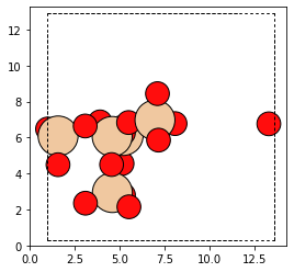
cluster, od = bea_zeolite.get_cluster(154)
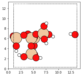
The cluster looks like this
plot_atoms(cluster)
the open defect looks like this
plot_atoms(od)
Both the open defect and the cluster are Zeolite objects, yet they
have a different ztype attribute
display(type(bea_zeolite))
display(type(od))
display(type(cluster))
maze.zeolite.Zeolite
maze.zeolite.Zeolite
maze.zeolite.Zeolite
display(bea_zeolite.ztype)
display(od.ztype)
display(cluster.ztype)
'Zeolite'
'Open Defect'
'Cluster'
Next we want to cap the cluster and changes some of the atoms its
structure. Capping involves adding hydrogens and oxygens to the cluster.
The built-in cap_atoms() method returns a new cluster object that
has hydrogen caps added to it.
capped_cluster = cluster.cap_atoms()
plot_atoms(capped_cluster)
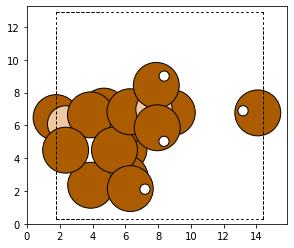
In a typical zeolite workflow, this cluster would be optimized. Configuring an optimizer can be tricky, and so for this tutorial we instead replace the oxygen atoms with aluminum atoms.
for atom in capped_cluster:
    if atom.symbol == 'O':
        capped_cluster[atom.index].symbol = 'Al'
plot_atoms(capped_cluster)
The next stage is removing the caps from the atom and reintegrating it back into the original zeolite.
To remove caps, we have to find the name of the caps in additions
dictionary
dict(capped_cluster.additions)
{'h_caps': ['h_caps_34']}
or we can just select the last h_caps added using pythons list methods
additon_category = 'h_caps'
addition_name = capped_cluster.additions[additon_category][-1]
display(addition_name)
'h_caps_34'
Next we call the remove_addition method
uncapped_cluster = capped_cluster.remove_addition(addition_name, additon_category)
plot_atoms(uncapped_cluster)

The caps have been removed. We can now integrate the cluster back into the original zeolite.
bea_zeolite_with_al = bea_zeolite.integrate(uncapped_cluster)
plot_atoms(bea_zeolite_with_al)
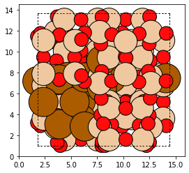
The changes have been made. An important thing to notice is that none of
the structural manipulation features of MAZE have side-effects. The
bea_zeolite remains unchanged by this integration and a new
bea_zeolite_with_al is created. Along with leading to cleaner code
with fewew bugs, this style of programming also allows for method
chanining.
This demo showed the power of the MAZE code to extract and add clusters to zeotypes. This is one of the most useful features in the MAZE code.